A fairly common problem I see motion graphics artists struggling to figure out in Houdini is how to animate objects procedurally, but have them collide realistically while moving. They want to be able to art direct the animation of objects using broad strokes, a pretty common pattern for mograph, but then make sure objects aren’t overlapping each other. This is trickier than it sounds! You can’t just apply a relaxation algorithm after the animation because it won’t be temporally consistent; the relaxation solve might differ between frames and cause objects to jump around and jitter unrealistically. The only good way to handle this is to run a full simulation, using the original animation as a guide.
There are two primary approaches you can take for guiding this kind of animation-driven simulation. (The Bullet RBD Solver has a “Guides” option but it’s designed to handle controlled destruction, not the kind of precise animation we’re after.) One approach is to compute forces that can translate and rotate your RBDs to match the motion from SOPs; this happens to be what MOPs Plus does in its various DOP nodes. If you want to do this on easy mode, MOPs+ Apply Attributes DOP handles everything for you. The other approach is to use soft pin constraints. Soft pins are great in that they can have varying stiffness, so you can control how rigidly the RBDs try to adhere to their constraint targets. The process of setting them up is a bit annoying, though, so I’m going to go over some of the nuances of building and then driving these constraints.
Example 1: Translating a single constraint anchor
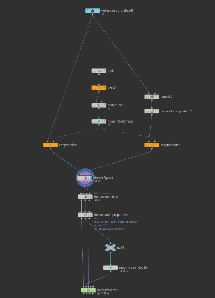
Here’s the starting point for a very simple example. I have two pig heads here, and I’m going to animate one of them colliding with the other. In the interest of getting more accurate (and faster) collisions, I’m creating proxy geometry by first remeshing the pig head, then running it through the Convex Decomposition SOP. This breaks the pig head down into multiple convex hulls that the Bullet solver will then treat as a single object. I then make the second pig head by copying the first (for both the original geometry and the proxy, via Reference Copy) and connect the result of each branch to the Geometry and Proxy Geometry inputs of the RBD Configure SOP. The network looks like this:
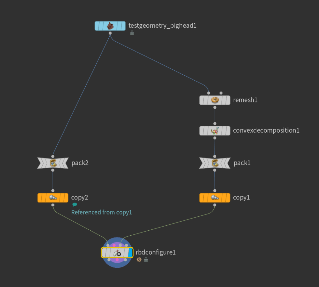
Just with the default settings, the RBD Configure SOP is going to ensure that our Geometry and Proxy Geometry have matching name attributes, and it’ll add any necessary physical attributes like density to the points of the Proxy Geometry (since that’s what’s actually being simulated). The name attribute is terribly important with RBD simulations, as each unique name defines a single object. Multiple primitives with the same name will solve as a single object! This can be a blessing or a curse; either way it’s something you need to be very aware of. The name attribute is also what links the Geometry to the Proxy Geometry, so that the transforms of the simulated proxies are copied back to the original geometry post-sim. Keep your spreadsheet open! You are not an effects artist if your spreadsheet is not visible at all times!
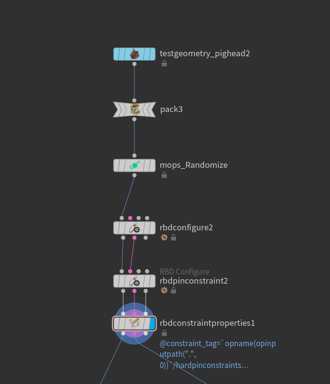
The next thing to tackle is creating the constraints. In past versions of Houdini this was much more annoying to do. It’s still annoying, but thankfully not as bad as it was. The RBD Pin Constraint in the Tab menu is a macro of sorts that will drop down a preconfigured RBD Configure SOP with some pinning presets applied, followed by a connected RBD Constraint Properties DOP. You could just enable Soft pins in the first RBD Configure DOP you made if you like, or skip the first RBD Configure and use the nodes given to you by the macro, it really doesn’t matter that much. Here’s what that network looks like now:
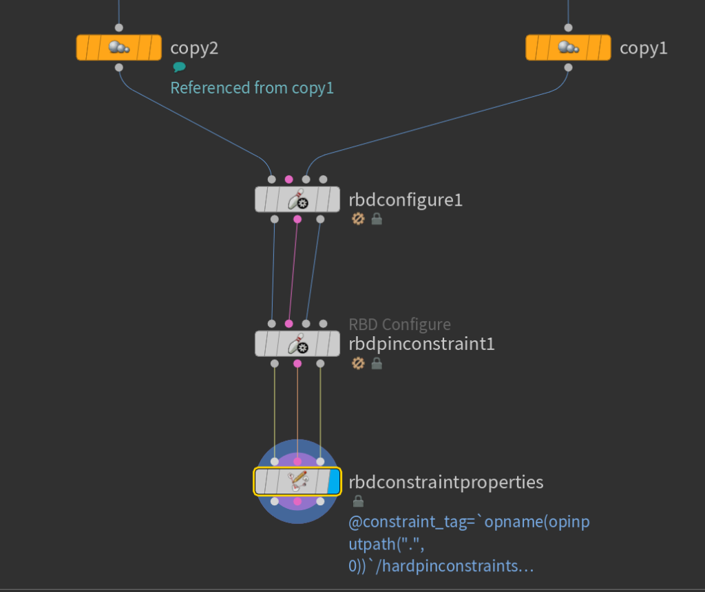
One obnoxious thing that this macro does, however, is default to Hard (Deprecated) constraints for the pins. Why a macro would default to a deprecated option is an interesting question, and one I’ll leave to future generations. For your purposes, just switch that Pin Type to “Soft” and the connected RBD Constraint Properties SOP will update as well.
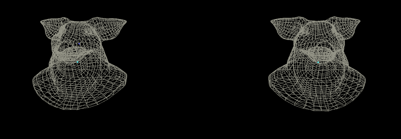
Now let’s actually see what these constraints are. All of these complex RBD configuration tools, in the end, are just creating two-point polygon primitives with some special attributes on them. If you drop down a Null SOP and wire up the input to the constraints output (the pink one in the middle), you’ll see that there’s just a couple points visible in the viewport. Look to the spreadsheet, and you’ll see that there’s actually four points: two overlapping points for each pig head. One point has a name attribute that matches the pig head that’s nearest; the other point has a blank name.
These name attributes are super important! Remember that RBD is all about names; that’s how it establishes what objects are. In the case of constraints, the name is telling you what object is constrained by the given point. The points that don’t have names are “world space anchors,” meaning they aren’t following any other RBD object in the scene. These little guys are the ones you’ll be animating.
Switch over to the primitive attribute view in the spreadsheet, and you’ll see that there are two primitives; one for each pair of points. You can’t see the connection between the points yet, but each constraint pair is connected by a single polyline primitive. This connection is how Houdini knows to associate each point. The spreadsheet also has all kinds of interesting attributes that are set up by the RBD Constraint Properties SOP. Here’s a few of the more important ones:
constraint_name: this is more or less a name used by other RBD nodes that hints at what kind of constraint we’re dealing with. If you’re doing an RBD setup entirely from scratch in DOPs, this can be whatever you want as long as it matches the name defined in DOPs, but with SOP RBDs these are predefined and you don’t need to worry about them too much.constraint_type: this defaults to “all”, meaning both position and rotation are constrained by the anchors. Adjusting the “Degrees of Freedom” parameter on RBD Constraint Properties will update this attribute to “position” or “rotation”.restlength: how far apart the constrained object should be from its partner object or world space anchor.stiffness: how badly you want Bullet to work to satisfy the constraint.
Don’t forget that you can muck around with these attributes any way you please before the simulation! If you don’t like the controls that RBD Constraint Properties gives you for managing stiffness or whatever, you can feel free to use Attribute Randomize or whatever you want to manipulate these values.
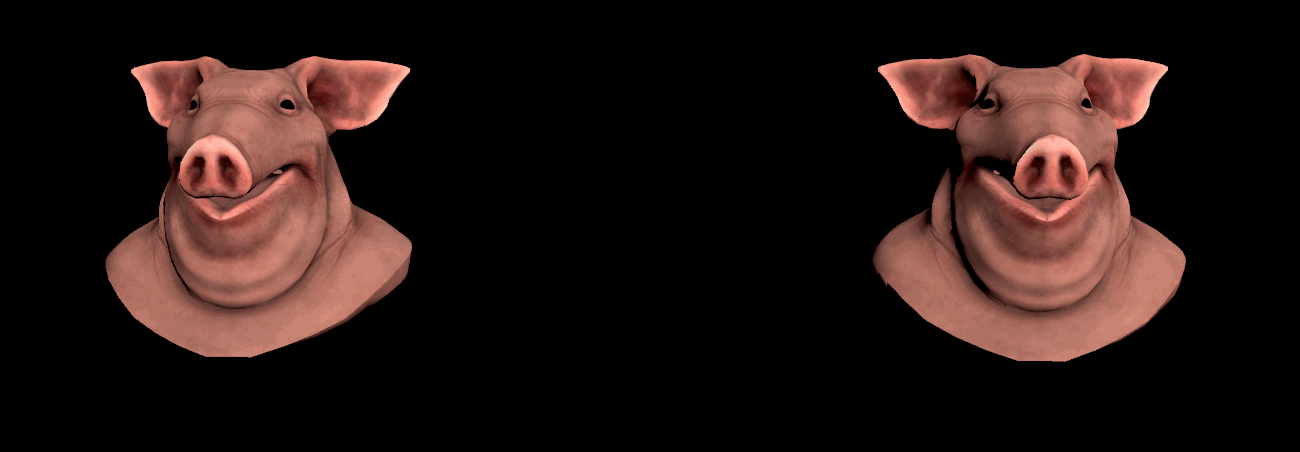
Now it’s time to animate this. Wire up a Transform SOP to the constraints output (the pink one) of your RBD Constraint Properties, and set the Group mask to 0 and the Group Type to Points. Point 0 is the point without a name, meaning it’s the world space anchor for the pig head on the left. Set a few keyframes (the horror!) to animate this point closer to the other pig head over a second or so. As you translate the world space anchor point, you’ll start to see the polyline primitive that connects the two constraint points.
Now that this is animated, we’re ready to simulate. Wire up the original geometry to the first input of an RBD Bullet Solver SOP, constraints to the second, and the proxies to the third. If you press play to simulate, you still won’t see anything happen despite our earlier keyframes. If you remember my previous blog post, the reason might be familiar to you: the P attribute that we’re animating here is not being updated during the simulation, because simulations by default only care about the initial conditions (the attribute values at the start frame of the sim). To correct this, go to the Constraints tab of the solver, scroll all the way to the bottom and look for “Override Attributes”. Add P to this field and play again, and you’ll see the pig head doing its best to follow the animated world space anchor:
Example 2: Orientation
It’s thankfully not too hard to throw orientation into the mix, especially with MOPs. Houdini can support rotating individual points natively, but you’ll need to initialize a valid orientation first by first using an Attribute Create SOP to create a point attribute named orient, setting the Size to 4 and the Value to {0,0,0,1}. This particular value is considered the “identity” rotation, basically meaning no rotation at all. You can then use the Transform SOP or the Edit SOP to handle the rotation of the point. With MOPs, you can just use MOPs Transform and it’ll create and adjust the orient attribute for you. Remember that since you’re animating a new attribute, you’ll need to add orient to the list of Override Attributes on the RBD Bullet Solver! Here’s the same animation with the same anchor point rotated a bit to modify the orient attribute:
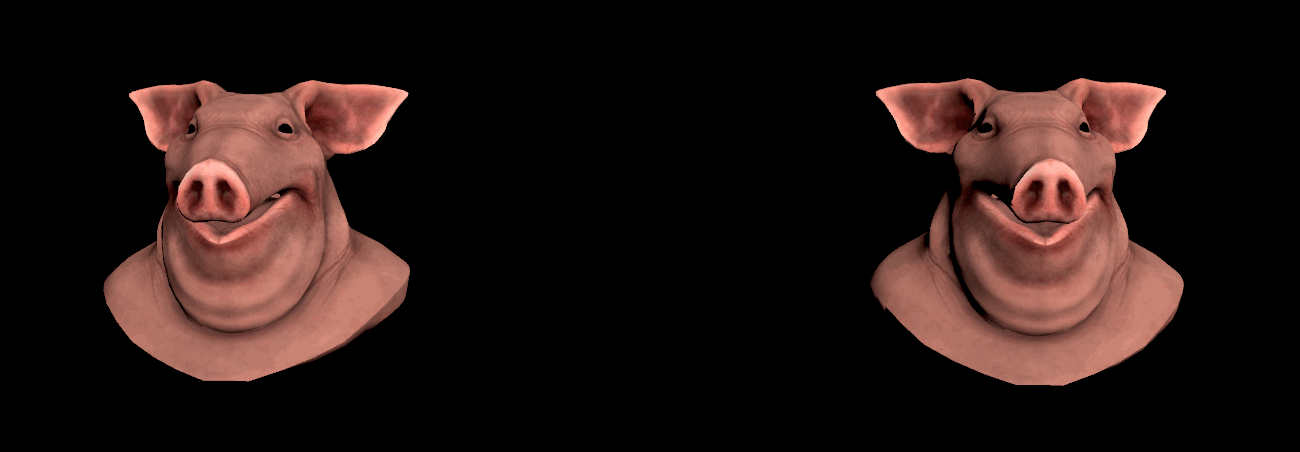
orient attribute as well as P on the world space anchor.Example 3: Morientation
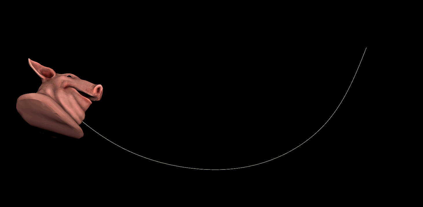
One more slightly more complex orientation example to demonstrate something interesting about these constraints. Here we’re starting with just a single pig head, packed and run through MOPs Randomize to scramble the orientation of the object. If you don’t want to use MOPs, you could use Attribute Randomize on the orient attribute in “Direction or Orientation” mode to accomplish the same effect. The RBD configuration and constraints are set up in exactly the same manner as before. Here’s the network:
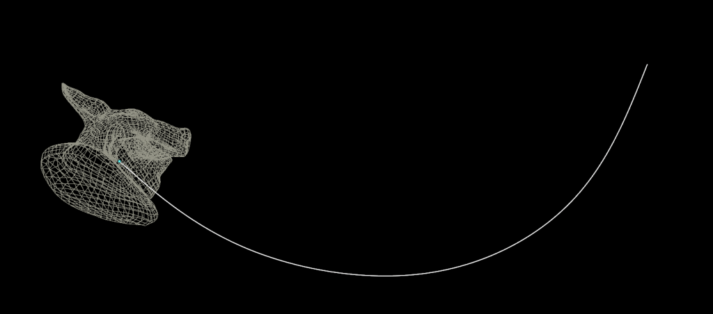
Now we’ll make things a little more interesting by drawing a curve that we want the pig head to follow. Use the second output of the RBD Constraint Properties DOP as the input to a Curve SOP, and the existing constraint point will be the first point on the curve (which is perfect because it also happens to be the starting position for our pig head to follow). Draw the rest of the curve, then append a Resample SOP and set Treat Polygons As to “Subdivision Curves” to smooth out the curve.
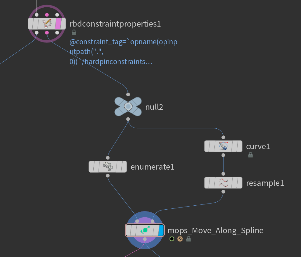
There are a few different ways we could animate this primitive along the curve here, but one of the easiest (surprise!) is MOPs Move Along Spline. MOPs generally likes points to have an id attribute, so first drop down an Enumerate SOP in Points mode and set the attribute to id, or just use a Point Wrangle with the code i@id = @ptnum; to create an id attribute. Then wire this to the first input of MOPs Move Along Spline, and the curve to the second input. Set the Group to 0 (the same world space anchor) and the Group Type to Points. Once this is linked up, all you have to do is go to the Animate tab of the MOPs node and animate the “Goal” parameter to move the anchor point along the curve. Your network should look like this:
If you wire up the pig head to the first input and your animated constraint points to the second input of an RBD Bullet Solver and then run the simulation (remember to update P and orient!) you will notice right away that something isn’t quite right… the pig head snaps into a very different orientation on the first frame of the simulation. What’s going on?

The problem here is a uniquely irritating one to Bullet, and will be familiar to anyone who has tried to create new constraints in Bullet mid-simulation. Constraint orientations are defined in local space, not world space! What we’re seeing here is effectively a “double transform”… the world space anchor orientation is trying to match that of the curve we drew (thanks to MOPs Move Along Spline!) but Bullet sees this as an additional transform to enforce on the constraint.
There are two ways we could address this. The manual way to do this is to determine the rest orientation from the starting frame of the animation and then “subtract” that orientation from the animating orientation so that we’re effectively storing the difference between the rest orientation and the animated orientation. The mathematical way to do this is to invert the rest transform and then multiply it by the current orientation (this gets us the delta between the two orientations). If you used a Timeshift SOP to freeze the animated constraint on the first frame and connected it to the second input of a Point Wrangle with the non-frozen constraint in the first input, the VEX would look like this:
// get the orientation from the first frame
vector4 restorient = point(1, "orient", 0);

// invert that orientation to "undo" it and get the difference
p@orient = qmultiply(p@orient, qinvert(restorient));
Of course, you could also just set “Maintain Orient Offset” to 1.0 on MOPs Move Along Spline, which will do this for you. Before we do this, a quick visual. Drop down a MOPs Visualize Frame SOP, or use visualizers however you like to show the orient attribute as the constraint moves along the path:
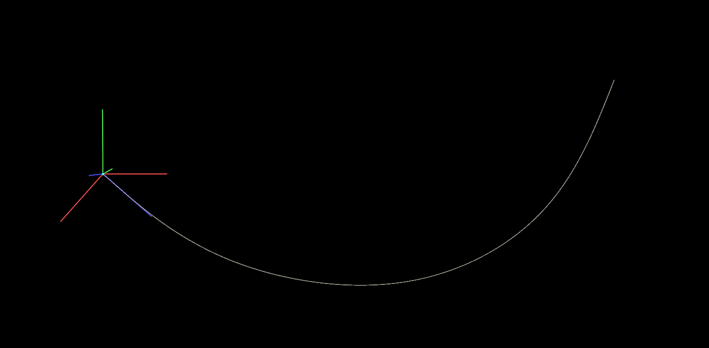
The constraint’s orientation is always facing the tangent of the curve, which is in most cases the behavior you want. But we want the constraint to start with a default orientation and only show the difference between the starting rotation and the animated one. By using either the VEX or the MOPs method to modify the orientation, the constraint looks like this:
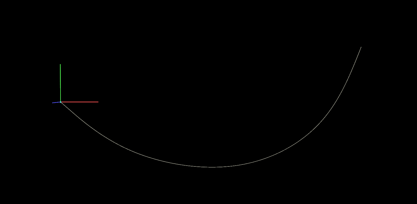
This is a really tough problem to wrap your head around! Hopefully visualizing it this way makes more sense of it. Once the constraint has been correctly defined in local space, the animation works as expected:
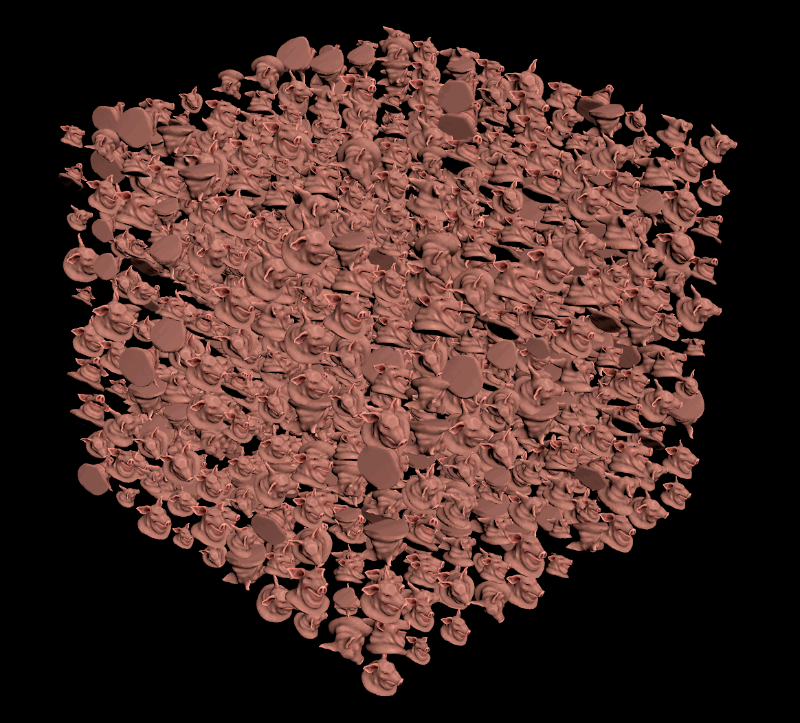
Example 4: MOAR CONSTRAINTS
Once you get how this setup is meant to work, it’s pretty straightforward to expand on it. Here I’m basically using the same proxy setup with convex decomposition as in the first example, but I’m copying the pig heads to a huge 3D grid of points instead, with the orientations and scales randomized. The pin constraints are set up in exactly the same way as before. Here’s the entire network:
In this example I’m having all the pig heads wander aimlessly by feeding all of the world space anchor points into the MOPs Noise Modifier. This handy little tool can affect both the position and the orientation of these points, and it can even seamlessly loop! Enable “Time Varying” at the bottom of the Noise Properties tab and the points will just start moving. To affect only the world space anchors, you can use the ad-hoc group mask @name="" so that only points without a defined name will be adjusted. Now all the pig heads will bounce about, but Bullet will ensure that the collisions are respected:
Hopefully this helps clear up one of the more confounding parts of Houdini simulations! Anything involving orientations is going to be headache-inducing no matter what, but with a bit of knowledge (and maybe some MOPs tools) it can be a much more approachable problem to solve.
Of course, I wouldn’t have you read this far without a HIP file, so here you go. The MOPs definitions should be embedded in case you don’t already have it installed so you can play around without having to mess up your local environment. Have fun!
2 Comments
Jim · 06/03/2024 at 14:35
Thank you!
Vlad · 10/30/2024 at 12:23
Nice, thank you for the article, very useful set-ups!