A Houdini RBD Primer, Part 1

Rigid Body Dynamics (RBDs) in Houdini have gone through a lot of changes in the last decade, and one side effect of all that rapid development is that there’s a lot of confusing legacy stuff left over in both Houdini and in outdated educational materials that I keep seeing new users get stymied by. SideFX have done quite a lot in recent years to make RBDs less painful than in the past, especially with their new SOP-wrapped workflows, but there are still some core concepts and points of confusion that tend to trip people up. I’m hoping this post (eventually series of posts…?) will help clear some of that up so that users just starting out with RBDs can have a better sense of what’s actually going on and how to set up a simulation a little more painlessly.

RBD and Bullet

As is typical with Houdini, there’s a lot of confusing terminology to get through right off the bat. When you start looking into RBDs, you’re going to see a lot of nodes that say “RBD” in them but they’re not necessarily what you think they are! If you never leave the SOP wrapped tools like RBD Configure and RBD Bullet Solver (and you often don’t need to go beyond those), this won’t be a problem, but if you’re in a DOP network trying to build a custom solution you can quickly get overwhelmed. Let’s get the basics out of the way:

Old DOPs (RBD Solver)

• RBD Object (RBD Hero Object)
• RBD Fractured Object
• RBD Point Object
• RBD Solver

New DOPs (Bullet Solver)

• RBD Packed Object
• Bullet RBD Solver
• Any RBD Geometry (SOP) node

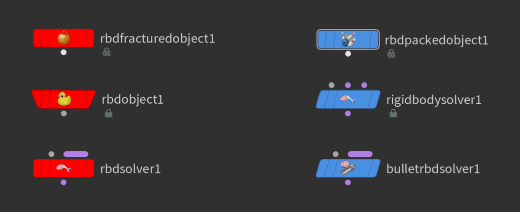
The RBD Solver in Houdini refers to a very specific (and rather old) volume-based rigid body solver in Houdini. If you’re the kind of person who uses shelf tools, you might have seen a little rubber duck icon named RBD Hero Object. This solver uses volumes for collisions and so it can be more appropriate, in some cases, for simulations that need to have complex interactions with fluids. 99% of the time, though, this is not the solver you want. It is far slower and more difficult to control than the alternative solver, the Bullet RBD Solver.

The Bullet RBD Solver is a third-party technology that’s been around for ages and is now the standard for rigid body simulations in Houdini. Houdini’s Bullet implementation uses packed primitives to define objects to simulate, and rather than expensive volume-based collision, Bullet uses convex hulls or primitive shapes like capsules, spheres, cubes, etc. to solve collisions. This simplification means Bullet can run much, much faster than the old RBD Solver.

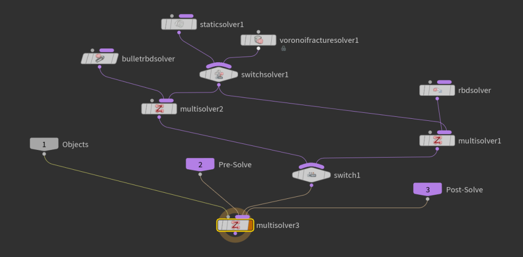
Confusingly, some of the nodes listed above are actually compatible with both the RBD Solver and the Bullet solver. If you click on the RBD Object DOP, for example, there is a tab for both RBD Solver attributes and Bullet data. The Rigid Body Solver DOP similarly can operate on either old school RBDs or on Bullet. If you unlock the node and dive inside, you can see that it’s essentially just a switch between the Bullet RBD Solver DOP and the RBD Solver DOP, wrapped in an interface for you.

Unless you know you need the “hero” RBD Solver, always default to Bullet / Packed RBDs.

For the rest of this article I’m going to be dealing with Bullet, because in practice that’s what almost every rigid body simulation you do, if not all of them, will be using. Ye olde RBD solver is very niche and rarely used and if you’re in a situation where you need it that badly, I’ll assume that you’re experienced enough with Houdini that you can dig through the example files and sort it out.

Packed RBDs

Whenever you’re dealing with the Bullet solver in Houdini you’ll often see the word “Packed” involved, and that’s because Houdini uses packed primitives (or packed fragments, a similar geometry type) to describe each rigid body. A packed primitive is represented by a single point with some attributes on it, some of which describe how to process the object for the Bullet solver. Packed primitives also include a transform “intrinsic” primitive attribute that describes the orientation and scale of each piece (the position is handled by the P attribute). Packed primitives are used all over the place in Houdini; they’re the basis of most instancing in Houdini and they’re also what MOPs primarily interacts with. For more information about packed primitives and transforms and all that, see my Instancing Guide.

Your fractured geometry (or whatever you’re simulating) is typically converted to packed fragments by the RBD Configure SOP. This uses the name primitive attribute on the existing geometry to identify pieces, and converts each named piece into a packed fragment. It also promotes the name attribute from the original primitives to the point representing each piece.

The name attribute is one of the most important and fundamental parts of Bullet that you need to understand. Bullet differentiates objects in the simulation based solely on name. If multiple packed primitives have the same name attribute, they will solve as a single object. This is both very powerful and potentially very annoying! If you accidentally create multiple pieces of geometry with the same name value, or more commonly, merge two geometry streams together with overlapping name values, Bullet will assume they’re the same piece and give you very unpredictable results:

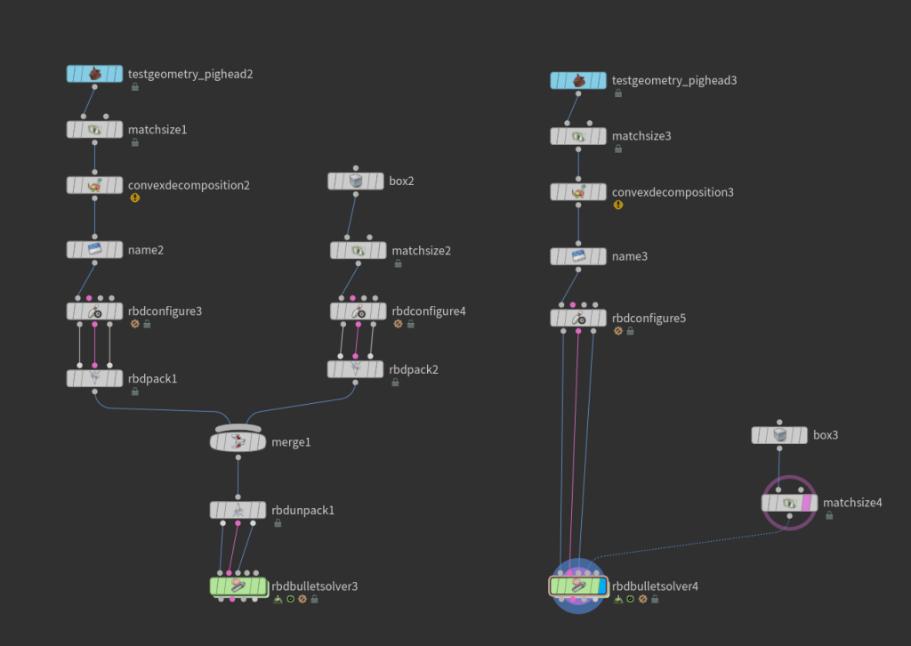
You can often avoid accidentally creating duplicate name attributes by using the RBD Pack SOP prior to merging objects together, and RBD Unpack SOP afterwards. RBD Unpack has an option to enforce unique name attributes on instances, and this can help you if you have multiple copies of the same fractured object being merged together. The other straightforward option is to edit the Name Prefix parameter on the RBD Configure SOP so that each object is guaranteed a unique name prior to merging.

Understanding how to manipulate the name attribute gives you the ability to break complex objects down into simple parts that are much easier for Bullet to solve. This brings us to the most common type of collision object that Bullet supports: convex hulls.

Bullet and Convex Hulls

A big reason why Bullet can move as fast as it does is because it takes certain mathematical shortcuts to determine whether or not objects are colliding with each other. Bullet supports a number of different collision shape types, shown under the “Collision Shapes” rolldown of the RBD Configure SOP as the “Geometry Representation” parameter. The default, and most common option, is “Convex Hull”.

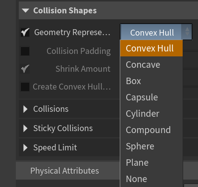
Bullet very much prefers convex geometry, including the basic primitive shapes like “Box” or “Capsule” that appear in this rolldown. Concave shapes force Bullet to make much more expensive (and frequently inaccurate) calculations during the simulation to test for collisions. It’s so much slower and unpredictable that in my opinion you should simply never use Concave collisions. Forget it’s there!

If you can’t quite visualize what “convex” means, just drop down a Pig Head SOP and then a Convex Hull SOP to illustrate it in clear terms:

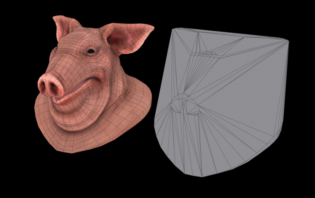
Since Convex Hull is the default for Bullet collisions, if you feed it packed primitives that have concave geometry like this pig head, you’re going to get imprecise collisions. Here’s an example using an L-shaped piece with just the default convex hull:

Now here’s the same simulation with the geometry processed into multiple convex hulls via a process called Convex Decomposition, conveniently handled by the Convex Decomposition SOP (and a Remesh SOP):

Note that prior to the RBD Configure SOP that sets all the physical parameters for this object, I’m using a Name SOP to give every primitive the same name attribute. When RBD Configure sees this attribute, it knows to create a single packed primitive for the entire object based on name, but Bullet will recognize the convex hulls inside and use them to create the collision representation. Note that this feature is only the default option when you’re using the SOP-wrapped Bullet tools… if you’re building the simulation the old-fashioned way in a DOP network, you’ll need to enable “Create Convex Hull per Set of Connected Primitives” on the RBD Packed Object DOP.

If I don’t set the name attribute, RBD Configure will give me one packed primitive for each convex hull, and I get this simulation instead:

If you take a look at the Collision tab of the RBD Bullet Solver SOP, you’ll see there’s a Collision Shape control here, too. If you don’t define a collision shape type in the RBD Configure SOP, this acts as the default. If you do define a collision shape type up front, Bullet understands this by reading the bullet_georep point attribute on your packed points. This allows you to mix and match collision primitive types; if you have a lot of roughly box-shaped objects colliding with a hero object, for example, you could speed up your simulation quite a bit by using box colliders for the boxes and convex hulls for the hero object. Get used to looking at these attributes! Always keep that spreadsheet open!

While we’re here looking at our collision representation, it’s extremely important to understand Collision Padding. If we take our packed primitives after the RBD Configure SOP and scale them down from meters to centimeters, check out what happens to the collision representation:

Bullet’s defaults like to think in meters; it was originally designed to handle destruction of things like brick walls. If you’re fracturing something very small, expect problems like this to arise. You can potentially correct for this by reducing the collision padding to a much smaller value, or you can just scale your scene up so that it’s at least a meter or two across, then scale back down afterwards. I know some purists will hate the idea of simulating at a non-real-world scale, but you have to understand that solvers have preferences and biases built-in, and it’s often way easier to just roll with those preferences than to try to fight the solver. Feel free to put me on blast in the comments but that’s just how it is.

Static Colliders

Another very common mistake for artists new to Bullet is thinking that static colliders (meaning passive objects that your simulation is meant to collide with) are in any way special or different compared to your simulated objects. This might be true in FLIP or POP simulations, but in Bullet, everything is convex hulls. This includes static colliders!

In practical terms this means that there’s no difference between how you prepare static colliders versus active objects. They all need to be represented by convex hulls or simple Bullet primitive shapes with name attributes that don’t conflict with each other (unless they’re meant to represent the same object). With the exception of colliders that move or deform, the only real difference between a static object and an active one is the point attribute i@active being set to 0 (static) or 1 (active).

If you’re in a DOP network and not using the wrapped RBD tools, this means that your static collider objects are not defined using a Static Object DOP; you’d use either a second RBD Packed Object DOP, or just merge the colliders in with the rest of the simulation, ensuring that i@active is zero on the static objects. Both methods are valid; the only difference with the latter method is that the DOP Import SOP will fetch the static colliders along with your active geometry since they’re a single DOP object.

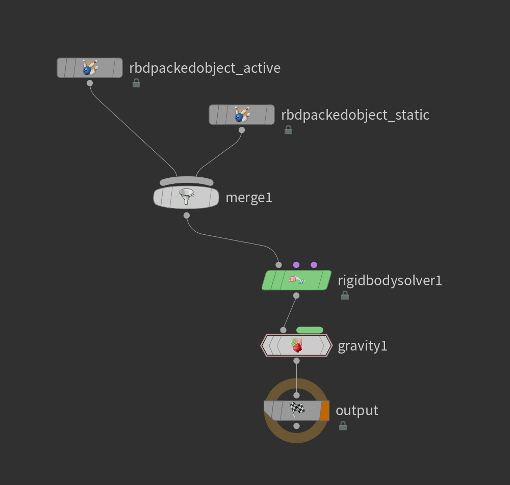
Deforming vs. Animated

What happens if your colliders aren’t just sitting there? In many situations the collider is animating. Bullet supports updating the collision representations of objects via two point attributes: i@animated and i@deforming. These attributes can be set via the RBD Configure SOP, or they can be set as defaults under the Collision tab of the RBD Bullet Solver SOP. The difference between these two attributes is important!

If i@animated is 1, Bullet will read the intrinsic transform attribute from each packed primitive in SOPs, and update the transform in DOPs to match. This is a pretty lightweight operation and is generally what you want when you have a moving collision object. If i@deforming is 1, however, Bullet will actually update the collision mesh for each packed primitive on each timestep.

Let’s look at a quick example to tie all this together. Here’s a simple collision object that’s twisting around. It looks like this:

Now let’s drop a ball on it. On the RBD Bullet Solver, set the Collision Type to Deforming. This forces the mesh to update on each timestep. Now take a look at the resulting simulation:

That bounce is kind of weird, right? Enable “Show Collision Shape” under the Collision Geometry rolldown of the Visualization tab of the RBD Bullet Solver and you’ll see the first part of the problem here:

You might have guessed this would happen, but Bullet is reading this deforming geometry as a single convex hull, causing the twisting shape to push the ball upwards as it rolls along. We need to decompose this into multiple convex hulls so that Bullet can properly understand it.

Using a Convex Decomposition SOP prior to the Twist SOP nets us this simulation:

This is better, but it can still be improved. While we’re getting the collisions we want, recomputing the deforming collision hulls on each timestep can be slow. In this particular simulation, it’s about 8.5 seconds of cook time for 5 seconds of animation. Not bad, but could be better.

For this particular collision object and many others, the deformation could be just as well described by some transformations, especially when the collider is decomposed into a reasonable number of chunks. Converting this deformation to transformation could be done by freezing a reference frame of the collider with a Time Shift SOP, packing the pieces into fragments, and then point deforming the fragments with the original animation, but there’s a lesser-known SOP that’s purpose-built for this sort of thing called RBD Deforming to Animated SOP. It’s not going to match the deforming geometry 100%, but in many situations it can get very close. After this SOP is placed we can go to the RBD Bullet Solver SOP and change the Collision Type from Deforming to Animated:

This cuts down the simulation time to 6.5 seconds, about 75% of the original simulation time. Doesn’t sound like much but on a much longer or more complex simulation, this extra time savings really adds up!

If you don’t want to spend quite so much time prepping all your collision geometry, there’s of course a MOPs node to help you: MOPs+ Collision Geometry. This handles all of the above prep work and will also apply it efficiently to instances, including animated instances like Alembic sequences, ensuring they’re all decomposed and animating as efficiently as possible.

Template Point Attributes

This is a “new” feature as of Houdini 19.0, but it was overlooked by a lot of people and didn’t exist when a lot of Bullet tutorials for Houdini were released. In the old days, if you wanted to use VEX to set the transform of an object in a Bullet simulation, the only way to do it was by manually setting the transform primitive intrinsic attribute. Even more esoteric, if you wanted to change the scale of a Bullet object during the simulation, the only way to do it was to both update the transform intrinsic but also set the id attribute of the affected point to -1, which was a secret code to force Bullet to recompute the collision geometry for that mesh. It was slow and kind of cumbersome to do this.

Now you can update transforms in a Geometry Wrangle DOP simply by setting template point attributes, just like you would with a Copy to Points SOP. The caveat here is that the template point attributes are going to be read *relative to the rest transform*, defined on the first timestep the object exists. Let’s try an example.

Here’s a bunch of boxes randomly floating above a ground plane and falling. Double-clicking on the RBD Bullet Solver SOP lets you apply custom forces, which include Geometry Wrangles. I’m dropping down a Geometry Wrangle and connecting it to the “PRESOLVE” output with the following expression:

if(@P.y <= 0.51) {
    @pscale *= 0.9;
}

This causes the boxes to shrink once they’re close to the ground:

Similarly, you could apply a constant rotation to the objects by updating the orient attribute. This isn’t the same as using POP Spin or some other force to cause the rotation, but in some cases it can be more controllable as the rotation will be immune to other forces aside from collisions. Update the code on the Geometry Wrangle:

// get local forward axis (local Z)
matrix3 m = primintrinsic(0, "transform", @primnum);
vector fwd = normalize(m * {0,0,1});

// rotate around this axis 10 degrees
float amount = radians(10); 
rotate(m, amount, fwd);

// convert this matrix to an orientation
p@orient = quaternion(m);

These transformations are done relative to the restxform matrix point attribute that’s generated on the first timestep of the simulation, meaning they’re in local space, not world space. Setting p@orient to the default, {0,0,0,1}, for example, will more or less just match the rest orientation at the first timestep.

There’s an important gotcha here: if your objects have template attributes prior to the simulation, they will be applied on the first timestep! For example, if your objects have @pscale = 0.1 set prior to the simulation, on the first timestep they’ll be scaled to 1/10th their original size as defined by the restxform attribute. If you use MOPs nodes like MOPs Randomize to arrange your objects prior to simulation, they will have template attributes, so be sure to delete those attributes prior to simulation!

If your goal is to make all of these transformations easy, consider using MOPs+ Transform DOP or MOPs+ Apply Attributes DOP, a couple of solvers you can use to easily art direct RBDs, Vellum, or other point-based dynamic objects without having to think about the math.

More resources

RBD is a really deep rabbit hole to go down, and this article is just surface-level stuff. You can get way weirder with this, especially when constraints are involved, but hopefully this is enough to get newer artists started with the core concepts of Bullet.

For some really great quick examples with HIP files included, I can’t recommend Nick Taylor’s article (and another more recent article) on Bullet enough, there’s really good stuff in there. I also have an article on using world space constraints to art direct RBDs, which might be helpful for understanding a bit more about how constraints work. I’m hoping to have a more detailed article on constraints later, stay tuned!