The rainy forest cinemagraph, Part 2

Continued from the previous post.

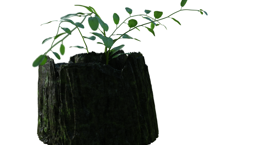
Part 2 here is all about the hero plant, which was by far the most time-consuming part of this whole process. The animation ended up being done primarily using FEM, which in retrospect was probably overkill. If I were to try this again, I’d probably try to build a more procedural system involving IK chains with maybe a layer of simple soft body dynamics on top to add springiness. Going the FEM route meant that each iteration took about 30 minutes to simulate, which adds up pretty fast. There are some neat little shortcuts elsewhere in the process, though, that hopefully some readers will find useful.

The hero plant

I am a masochist so I again started with L-systems to create the basic plant structure. L-systems are one of those things that start very simple and quickly build in complexity until they’re totally unreadable, so you generally want to keep notes of what the rules are actually doing as you build them. Of course, the notes from the original .HIP file that I posted are outdated, as they apply to an older version of the plant, so if you’ve already checked out the .HIP you may want to read these more accurate notes.

Here’s what the rules look like:

Premise: ~(20)a(“Cd”,1,0,0)FFX(c)$[+Y][-Y]
Rule 1: X(h): (h>0) = ~(d)TFX(h-1)
Rule 2: X(h): (h=0) = /(180)[^Y]FX(c)
Rule 3: Y = “Ta(“Cd”,0,0,0)F : 0.9
Rule 4: Y = “Ta(“Cd”,0,0,0)a(“dead”,1,0,0)H : 0.1

Okay, a bit complex-looking. There are a few layers in play here. The goal at its simplest here is to grow mostly upwards, twist a bit randomly, and droop a little to simulate gravity. Every few steps, a leaf should grow, from opposite sides of the stem (this is sometimes called an “alternate distichous” leaf pattern). The plant should always have a pair of leaves at the very tip, and there should be some random chance of leaves not growing at all (leaving a little nub behind). The stem points are colored red, while the endpoints are black, and the leaves that don’t grow are marked as “dead” with an attribute.

To break this down further: the premise starts with a random bend/twist (~(20)), defines the color as red (a("Cd",1,0,0)), grows upwards a bit (FF), creates the starting point for the function X (used in rules 1 and 2) with a value of c, which corresponds to “Variable c” in the Values tab, sets an up vector for the last leaves at the tip ($) so that they don’t grow perpendicular to the ground plane, then branches off and makes the two leaves using the function Y ([+Y][-Y]), which is defined in rules 3 and 4. That’s just the premise!

Rule 1 is defining what “X” means if the “counter” variable is greater than 0. You can see in the premise that we’re starting with X(c). “c” in the rulesets here refers to “Variable c,” which is set to 3. This means that at the beginning, our value for “h” within the context of these rules is 3 until modified later. The rule itself just wiggles randomly, using “Variable d” as a maximum amount, then applies gravity (T), grows forward a bit (F), then makes another function X at the end, but with 1 subtracted from “h”. Every generation, we subtract 1. This means that every third generation, we’re going to run Rule 2, where h=0.

Rule 2 is pretty simple. Twist 180 degrees (/(180)), branch off, pitch forward and create a Function Y, which is the “leaf” function (rules 3 and 4), then just keep growing up, resetting the counter to the default value “c”. What this means practically is that every third generation, we’re going to get a leaf, on the opposite side as the previous leaf.

Rules 3 and 4 grow leaves. They look more complex than they are. The " operator simply tapers the width of the stem, and then the attribute “Cd” (color) is set to black, for visualization purposes and to help with cleaning up geometry later. Then the leaf stem is grown and the branch stops. The two rules are almost identical, except that 10% of the time (the :0.9 and :0.1 are probabilities), the stem only grows half the usual length (H) and it’s given the point attribute “dead”.

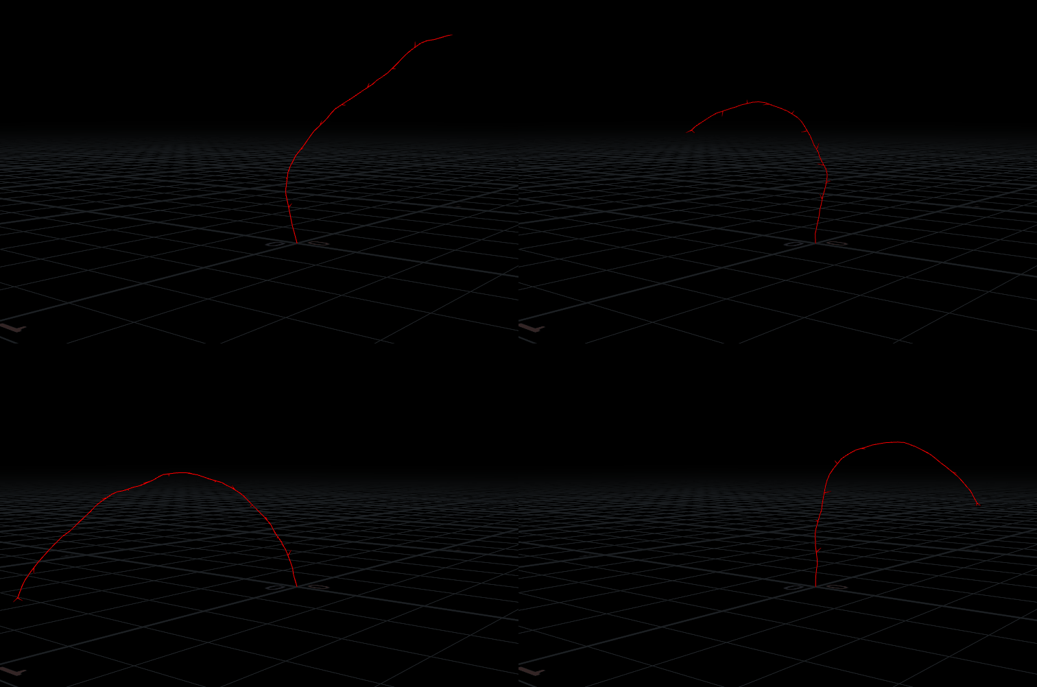
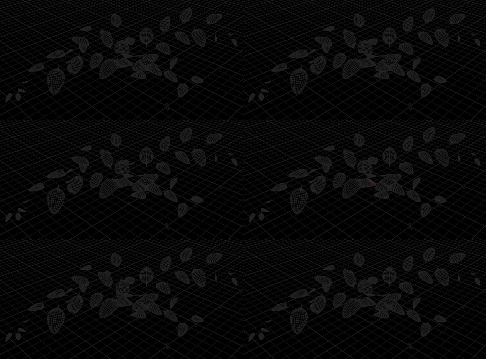
After this system was set up, I just sifted through different seeds and found four that looked pretty good. Here they are so far:

The four L-system seeds used for the hero plant.

There’s a bit of cleanup here, and then we get to some VEX. It was tricky to get the instanced leaf geometry to accurately connect with the stem geometry in a procedural way, so I needed to be able to shrink the stem “nubs” down. I also wanted some interactive control over the stem width across the length of the plant. To do this, I promoted the “arc” attribute generated by the L-system SOP to a detail attribute set to “maximum” so I could get a percentage value of the total arc length at each point, for use with a ramp parameter. Here’s the code:

float u = (float)@arc / detail(0,"maxarc",0);
@width = chramp("width_ramp",u) * ch("width_scale") * max(@Cd.x,0.5);
// if the point isn't red, it's a leaf stem, so shrink it

// isolate start and end points
if(( neighbourcount(0,@ptnum) < 2) && @dead == 0) {
    @group_ends = 1;
}
if(@ptnum == 0) {
    @group_ends = 0;
    @group_start = 1;
}

The width attribute is blurred afterwards to smooth out transitions a bit, and then a similar VEX setup is used to generate values for @targetstrength, to be used later in the FEM simulation. The leaves to be copied are treated in a similar way; a @targetstrength attribute is generated based on the position of each point along the length of the leaf, so that areas nearer the tip are less stiff. Before copying the leaf geometry to each “ends” point, the leaves are randomized slightly. Their scale is multiplied against a slightly randomized value, and also multiplied against a scalar based on which L-system generation they were created in, so that newer leaves near the tip of the stem are smaller than leaves towards the base. The “up” vector of each leaf point is also set to {0,1,0}, so they are more predictably aimed towards the sky when copied. The VEX looks like this:

// randomize attrs based on gen

float max_gens = ch("max_gens");

float base_scale = fit01(rand(@ptnum),0.5,0.75);
float scale_mod = chramp("leaf_scale_ramp",fit(@gen,1,max_gens,0,1));
@pscale = base_scale * scale_mod;
@N *= -1;

// point towards sky
v@up = {0,1,0};

The reason there are four randomization nodes here is because there are four specific L-system nodes that are generating the structure, and they each have a different number of generations. As shown later on, the simulations are run inside a Wedge ROP so that each plant is simulated by itself, and it was simpler to just have a Switch SOP used to control which plant is simulated for each wedge. It would be nicer to have this work completely procedurally, but some art direction was needed here in picking exactly which L-system seeds were used, and this seemed like the simpler way to go. Finally, the leaves are copied onto their respective stem points.

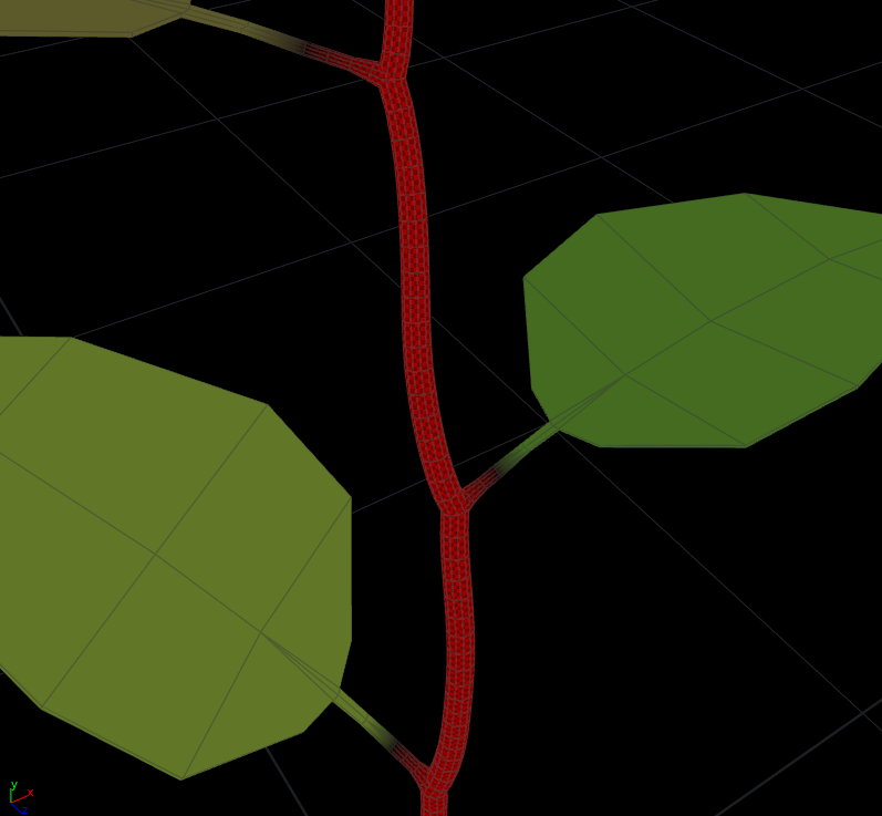
On the stem side, before merging with the leaves, there’s some processing to do. The Polywire SOP is convenient for building geometry on L-systems wires, but it tends to create pretty bad UVs and some questionable topology in places. Instead, the Sweep SOP is used for each primitive (the stem is one primitive, and each leaf nub is its own primitive) in a For-Each loop in order to generate exactly the geometry we want. The setup can be a little confusing, but here’s the gist of it: The stem primitive is given point UVs based on the arc length of each point divided by the total arc length. The cross-section primitive, a simple circle, is given vertex UVs. The backbone UVs are running in the “u” direction, and the cross-section UVs are in the “v” direction (hence the Vertex Wrangle setting @uv.y = @uv.x). It’s essential for this setup that the backbone for the Sweep SOP is using point UVs in U, and the cross-section is using vertex UVs in V. With these two inputs fed into the Sweep SOP, our mesh and UVs look pretty good! Before merging with the leaves, the open edges of the stem that are to connect to the leaves are grouped. The leaf edges are similarly grouped. After merging, the PolyBridge SOP is used to connect these groups together by a ring of polygons. It’s not perfect topology, but it’s good enough for this case.

Not bad for procedural?

Some more prep work before going to DOPs. A bounding box is used to group some points near the root of the stem. These points are given the attribute i@pintoanimation=1, which the FEM solver recognizes by default. This will anchor the stem to its current position. The geometry is also split into two branches here: one for simulating (the left side), and the other for deformation by the simulation (the right side). FEM supports “embedded geometry,” which means that we can run the simulation itself on low-resolution geo but use it to accurately deform more detailed geometry. On the left side, we first use the Solid Embed SOP to convert the low-resolution geo to tetrahedrons for use by the FEM solver, and then two more FEM-specific attributes are defined: @stiffness and v@targetP. The stiffness attribute is a multiplier on the several types of Stiffness parameters on the Solid Object DOP, and targetP defines the “goal” position for each point, so that the plant can try to maintain its default shape.

Finally, time to simulate! This took forever to balance. The attributes on the Solid Object aren’t really based on any kind of intuitive unit, so there’s some guessing involved. There was a lot of back-and-forth on the Stiffness Multiplier, To save time on iterations, collisions were disabled altogether. In “reality” the leaves are being impacted by raindrops, which would imply colliding with particles, but collisions are often slow to solve, and then the “feel” of the leaf impacts becomes dependent on the motion of the rain, which might not have the right “feel” in itself, and then a horrible feedback loop starts where you’re constantly trying to balance one against the other, wasting hundreds of hours. Instead, a better approach is often to solve the more massive objects first, and then use that simulation to drive the less massive objects downstream.

In that light, inside the DOPnet you’ll notice the Solid Object DOP is plugged into a Multisolver. Before the actual Finite Element Solver is run, there’s a SOP Solver in play. SOP Solvers are a fantastic tool, as they allow you to modify simulations as they run using the much more familiar SOPs context. In this particular solver, there’s only a few nodes. First a @density attribute is computed, which is used to scatter points on areas of low @stiffness. The Scatter seed is modified by both @Time and by a custom attribute which is bound to the input channel of the Switch SOP used to differentiate the plant L-system seeds. This is to make sure that each plant is impacted slightly differently. Finally, the “impacts” are generated by using these scattered points to apply a downward force to the leaves, via the v@fexternal attribute recognized by the FEM Solver. Here’s some VEX:

float chance = ch("chance");
v@fexternal = 0;
@Cd = 0;
if(rand(@Time*ch("seed")) < chance && (@Frame < 1220) && (@Frame > 1001)) {
    float rad = ch("radius");
    vector P2 = point(1,"P",0);
    float dist = distance(@P,P2);
    float falloff = chramp("falloff_ramp",fit(dist,0,rad,0,1));
    
    float forceamt = fit01(rand(@Frame),ch("force_min"),ch("force_max"));
    vector force = set(0,forceamt*-1,0);
    v@fexternal += (force * falloff);
    @Cd = falloff;
}

Essentially what’s happening here is if we’re between frame 1001 and 1220 (so that no impacts happen right at the end, which would break the looping effect), a random amount of downwards force is generated. This force is multiplied by a falloff value based on the distance between the scattered impact points and the currently sampled point on the leaf. Running that simulation gets us something like this:

The tetrahedrons output from the FEM simulation.

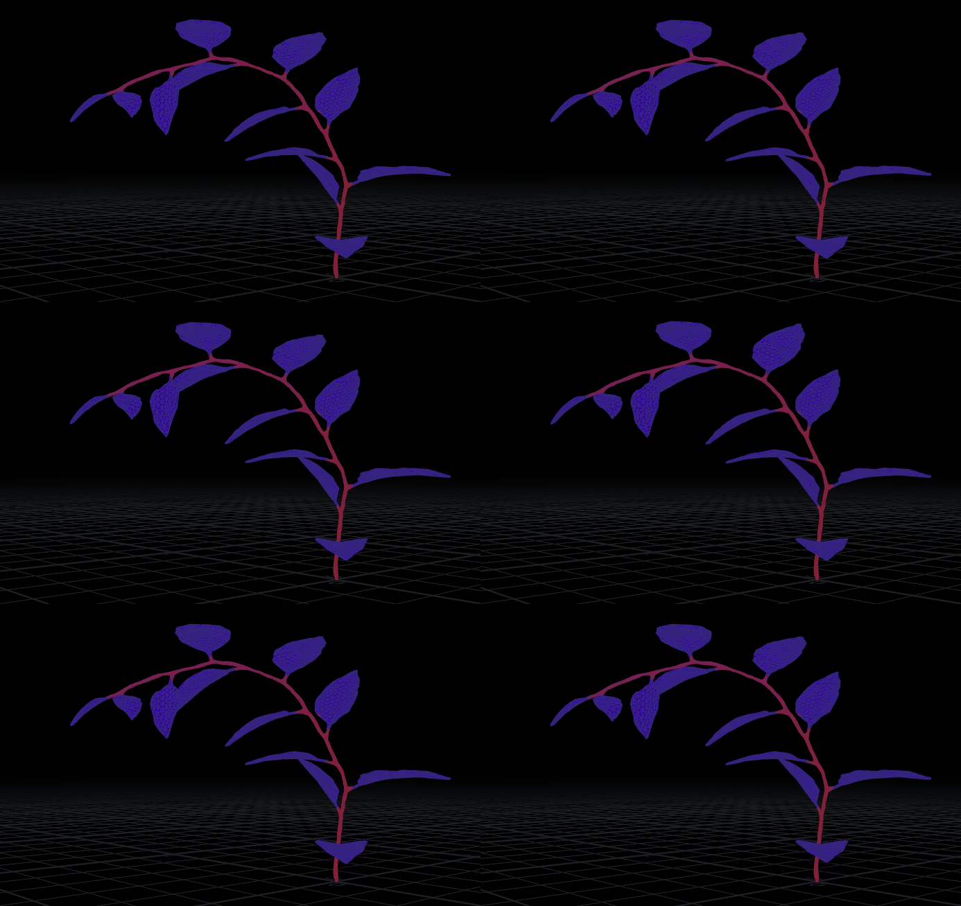
This is run four times, once for each plant variant, via the Wedge ROP. Inside ropnet1 there’s a Wedge ROP and a Geometry ROP. The Geometry ROP caches the results of the DOPnet to $HIP/geo/hero_plant_wedges/hero_plant_type_${WEDGENUM}.$F4.bgeo.sc. That ${WEDGENUM} magic in there is used by the Wedge ROP to make sure each plant type gets written out separately. The Wedge ROP is given a single parameter to modify, which is the Switch SOP’s input parameter. The other switches are connected to this first one, so each of the four plant types will get its own unique simulation.

There’s a couple of other tweaks to the leaves made downstream… the leaves are subdivided and then wrinkled up using some noise, then run through a Point Deform based on the original geometry. An extra UV set is also generated, mostly as a hack to try to have some more control over the sprite texture applied to the leaves without distorting the existing diffuse texture or causing other problems. For the most part, though, that’s it for the leaves. The material is an otherwise unremarkable subsurface shader with a texture applied as a Sprite cutout (again, this was a pretty bad idea, and you shouldn’t consider doing this to non-card geometry unless you’re desperate). Making leaf textures procedurally was going to take longer than I was willing to spend on this, so the textures are modified from some photographs:

The diffuse, normal, and alpha leaf textures.

The rain simulation

Most of the rain involved here is very simple particles, but the rain hitting the leaves needed to have a few extra fixins to make it believable. Since the impacts on the leaves from the previous FEM simulation weren’t driven by any “real” impacts, instead they had to be generated some other way. The easy way here was to get the length of the v@fexternal force we created in the earlier SOP Solver, and use that to create a mask from which we would emitter rain spatter. The mask attribute was called @forcemag and generated with this VEX:

f@forcemag = chramp("force_ramp",fit(length(v@fexternal),ch("min"),ch("max"),0,1));

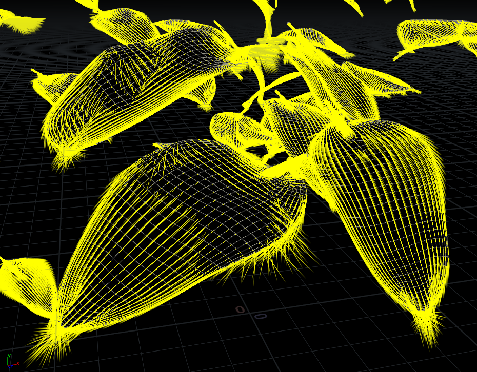
Basically the same exact pattern used to make the force in the first place. Set a minimum and maximum, bind it to a ramp parameter for easy tuning, and use the ramp to set the attribute. Visualizing this attribute nets us this:

The leaves with the @forcemag attribute visualized to show the points of impact.

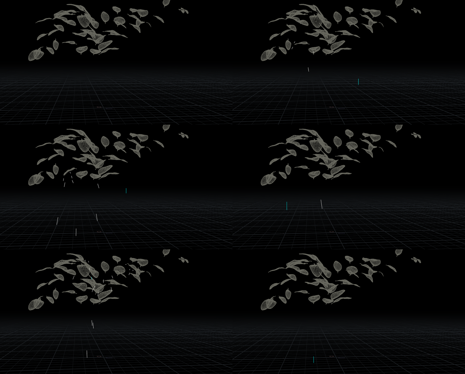
In order to generate emission points, we just need to blast primitives where @forcemag is below some threshold, and scatter points on the remaining primitives. These points are fed into a POP Object DOP in the next simulation, and create some short-lived rain spatter particles that fly upwards from the impact points. If we run the resulting particles through a Trail SOP afterwards, we get these little streaky particles:

The rain spatter after a Trail SOP.

The trickier part is figuring out how to get the droplets to stick to the leaves and run down their surfaces, like there’s some surface tension at play. This involved a fancy-sounded algorithm called gradient descent. Gradient descent allows us to try to find the most plausible path “down” the leaf, to give our raindrops that happen to stick to the leaf a sort of guide for which direction to move in. The guide will be written to the leaf points as the attribute v@tangent. The VEX for this algorithm looks like this:

int npts[] = neighbours(0, @ptnum);
vector pos;
float min = 99999;

for(int i=0; i<len(npts); i++) {
    vector p = point(0, "P", npts[i]);
    if(p.y < min) {
        min = p.y;
        pos = p;
    }
}

v@tangent = normalize(pos - @P);

Here’s what’s happening. First, we find all of our current point’s “neighbours,” meaning points connected by primitive edges. A couple of variables are initialized: a position vector, which will be the direction we eventually write to v@tangent, and a minimum value that we initialize to a very high value so that the minimum we find will certainly be smaller. Next, for each neighboring point, we get the position of that point, and see if its Y position is less than our minimum. If it is, we store it as the new minimum, and store its location to the position vector. In short, we find the lowest neighboring point. Finally, we write v@tangent as a normalized vector pointing to the lowest neighboring point. That’s it! Sounds more complicated than it is. Some filtering and blurring of these tangents is done afterwards, to prevent jittery results, since this algorithm is far from perfect especially when the leaves are in motion.

The leaf tangent vectors generated via gradient descent, visualized as yellow lines.

Now it’s time to add these sliding raindrops. From the earlier rain spatter particles, a few particles are randomly selected to be “stuck” and given the point attribute i@stuck to reflect this. The POP Solver recognizes this attribute and will try to keep the particle attached to the surface it’s stuck to, based on three other attributes: i@posprim (the primitive number to stick to), v@posuv (the parametric UVs of that primitive to stick to), and s@pospath (the SOP with these primitives). If you’re not sure about parametric UVs or any of that magic, take a look at this post about the magic functions xyzdist() and primuv(). After defining all of these attributes, the velocity is set to 0 and the lifespan is set to 10, so that the droplet doesn’t die out before it can fall off. The VEX looks like this:

// randomly set "stuck" behavior on particles
if(rand(@id+ch("seed")) < ch("thresh")) {
    i@stuck = 1; 
    int posprim;
    vector primuv;
    float dist = xyzdist(1,@P,posprim,primuv);
    // define stuck position
    i@posprim = posprim;
    v@posuv = primuv;
    @P = primuv(1, "P", posprim, primuv);
    s@pospath = chs("sticky_path");
    v@v = 0;
    // extend particle lifespan
    @life = 10;
    
}

What this means is that for the particles chosen to be sticky, as soon as they’re born we get the nearest position on the leaf surface using xyzdist(), and from that same function we can get the nearest primitive and parametric UV. We then bind all of these values, plus a parameter pointing to the leaf SOP (“sticky_path”) to the attributes the POP Solver is looking for (v@posuv, i@posprim, s@pospath) in order to facilitate sticky behavior.

Next, we have another POP Wrangle that slides the particles down the leaves. Here the v@tangent attribute we created earlier comes into play. This Wrangle uses point cloud functions to average the v@tangent value of the leaf points surrounding each particle, then uses it as a force to push the particle down the surface of the leaf. The amount of force is modified by the normal of the leaf points relative to the world up axis, using the dot product. Finally, after moving the particle along this vector, the particle is snapped back to the nearest point on the leaf. Here’s the VEX:

int posprim;
vector primuv;
float dist = xyzdist(1, @P, posprim, primuv);

vector N2 = primuv(1, "N", posprim, primuv);

// lookup tangents to compute vel dir
int max = 20;
float rad = 0.2;
int handle = pcopen(1, "P", @P, rad, max);
vector tangent = normalize(pcfilter(handle, "tangent"));

// mult velocity by dot product vs up
vector up = {0,1,0};
float mult = max(0.1, abs(dot(up, N2))) * 0.03;
vector v = tangent * mult;
vector pos = @P + v;
dist = xyzdist(1, pos, posprim, primuv);
@P = primuv(1, "P", posprim, primuv);
i@posprim = posprim;
v@primuv = primuv;

In writing this, I realized that the line where I’m using the dot product is probably actually doing the opposite of what I’d intended; I wanted the velocity to be reduced when the normal of the leaf points were facing straight up (so dot(up, N) would be 1), and at full speed when the normal and up vectors were orthogonal to each other (dot(up, N) would be 0). What I probably should have done was change that line to

float mult=max(0.1, 1-abs(dot(up, N2))) * 0.03;

or something like it in order to make droplets move much slower on a horizontally-oriented leaf. Oops! It still looks plausible as-is but I thought it was worth mentioning here that this did not actually work as intended and it’s just dumb luck that it still feels right.

Finally, there’s one more POP Wrangle used to release stuck particles. There’s two ways a stuck particle can release in this case: if the speed of the particle is above a certain threshold, or if the particle ends up running off the back of the leaf instead of the tip. The stems aren’t part of this simulation and I didn’t want to deal with trying to figure out how to stuff them into this calculation, so it was easier to just unstick any particles that happened to run in this direction. I’m lazy. Here’s the VEX:

vector vel = v@pprevious - @P;
@speed = length(vel);
// release particles above velocity threshold
if(@age > ch("min_age")) {
    if(@speed > ch("release_speed")) {
        i@stuck = 0;
        @Cd = {0,1,1};
    }
}
// release particles near leaf stems
if(inprimgroup(1, "bridgemeshprims", i@posprim)) {
    i@stuck = 0;
    @Cd = {0,1,1};
}

Taking these new sticky particles and running them through a similar Trail SOP setup creates a pretty nice effect:

The rain simulation with the “sticky” droplets added.

A little bit more processing, and we’re done. Once we’ve trailed all of our raindrops and used the Add SOP to connect them into solid lines, each trail is resampled and run through a For-Each loop to give each streak a characteristic “raindrop” shape. It’s easy enough to take an ordered polyline primitive and set a @pscale attribute on the points based on the point number of each point:

float u = @ptnum / (float)@numpt;
@pscale *= chramp("scale_ramp", u) * ch("scale_mult");
@pscale *= fit01(rand(i@sourceptnum), 0.5, 1.25);

That (float)@numpt, by the way, is necessary because both globals @ptnum and @numpt are integers, so we won’t get a nice 0-1 value for mapping to a ramp parameter unless we cast @numpt as a float first. Each trail also has another scale multiplier based on the age of each particle, so the trails of short-lived particles shrink and fade out instead of just vanishing. Once all the scale attributes are set up, the raindrops can be quickly meshed into renderable geometry via VDB From Particles. The original velocity from the particle sim is transferred back onto the meshed geometry for motion blur, and we’re done.

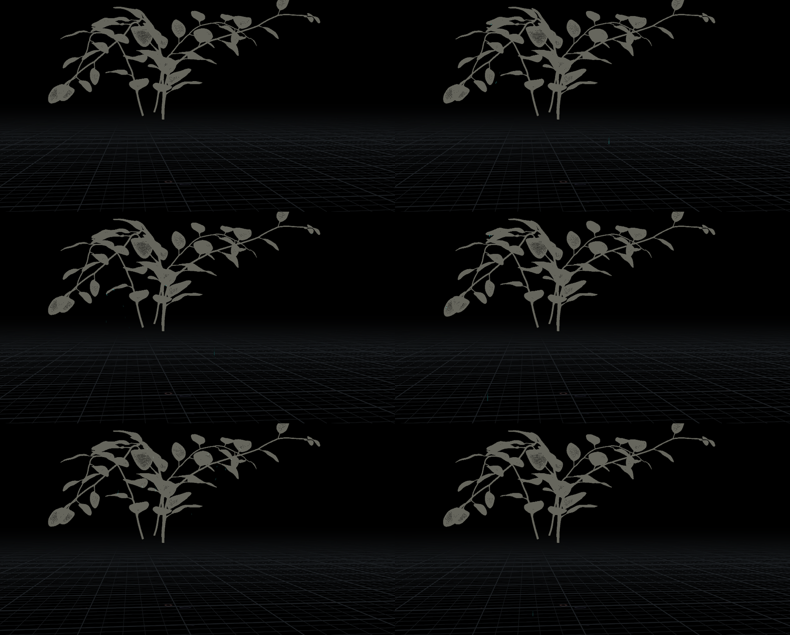
Here’s what the final simulation data looks like:

The final simulation.

That about wraps this up! Part 3 will go into the sprouts in the background and some of the other finer details. Feel free to leave questions or comments here, and please let me know if I have any glaring errors or omissions. Next post coming soon!